Processing Tools
The Processing menu collects GeoLibre's analysis and conversion tools. It holds two separate toolboxes (why), plus the SQL Workspace, Python Console, AI Assistant, and AI Segmentation, which have their own pages.
Two toolboxes in one menu
This is the single most common source of confusion in the Processing menu, so it is worth reading before anything else.
The menu is laid out like this:
Processing
├─ AI Assistant
├─────────────────────────
├─ Whitebox Toolbox        ← opens the toolbox dialog
├─ Conversion       ▸  ┐
├─ Hydrology        ▸  │
├─ LiDAR            ▸  │
├─ Network          ▸  │
├─ Projection       ▸  ├  the same toolbox, browsable
├─ Raster           ▸  │  by category (1,000+ tools)
├─ Remote Sensing   ▸  │
├─ Terrain          ▸  │
├─ Vector           ▸  ┘
├─────────────────────────
├─ GeoLibre Toolbox ▸      ← GeoLibre's own built-in tools
│   ├─ Conversion         ▸
│   ├─ Vector             ▸
│   ├─ Network            ▸
│   ├─ Spatial Statistics ▸
│   ├─ Raster             ▸
│   ├─ DGGS               ▸
│   ├──────────────────────
│   ├─ Geocode Addresses
│   ├─ Batch & Models
│   ├─ AI Segmentation
│   ├─ Object Detection
│   └─ Segment Everything
├─────────────────────────
├─ SQL Workspace
├─ Python Console
├─ Jupyter Notebook
├─ Dashboard
├─ History
├─ Planetary Computer
└─ Earth Engine
The block between the first and second separators belongs to the Whitebox Toolbox; everything under GeoLibre Toolbox is GeoLibre's own. Because both toolboxes cover vector, raster, conversion, and network work, several category names appear twice. They are not duplicates, and they do not open the same thing:
| Whitebox Toolbox | GeoLibre Toolbox | |
|---|---|---|
| Where in the menu | The Whitebox Toolbox item and the nine category submenus directly below it | The GeoLibre Toolbox submenu below the separator |
| What it contains | 1,000+ tools: the Whitebox Next Gen suite plus GeoLibre's own Rust tools from geolibre-rust | GeoLibre's built-in tools, written for this app |
| Categories come from | The tool manifests, generated automatically | Hand-curated for this app |
| What clicking a tool opens | One shared dialog, with the tool preselected and its form built from the tool's parameter manifest | A purpose-built dialog per tool family (Vector tools, Raster tools, Conversion, …) |
| Where it runs | WebAssembly in the browser by default, optionally the Python sidecar | Turf.js or Pyodide in the browser, or the Python sidecar, depending on the tool |
| Input | A map layer or a file | Usually a layer already on the map |
The two paths that look alike
The pair that trips people up most often:
Processing → Vector → GeoLibre (WASM)lists the several hundred vector tools GeoLibre contributes to the Whitebox toolbox. They are compiled from geolibre-rust to WebAssembly and sit in the same catalog as the Whitebox Next Gen tools, so the menu groups them under aGeoLibre (WASM)subheading to show where they came from. The same subheading appears under Conversion, Raster, Hydrology, and LiDAR. Every one of these opens the Whitebox Toolbox dialog.Processing → GeoLibre Toolbox → Vectoropens GeoLibre's own Vector tools dialog: buffer, clip, spatial join, and the rest of the list below, with an engine picker (Turf.js, GeoPandas sidecar, or Pyodide).
So the first is "the vector part of the Whitebox toolbox, filtered to the tools GeoLibre wrote", and the second is "GeoLibre's own vector toolbox". Both exist because they are different implementations with different strengths, not because one is a copy of the other.
A few individual tool names collide the same way. Processing → Conversion → GeoLibre (WASM) → Vector to PMTiles is a WASM catalog tool that opens the Whitebox Toolbox dialog; Processing → GeoLibre Toolbox → Conversion → Vector to PMTiles is the Conversion dialog documented below, with its own file pickers and zoom, compression, and layer-name options. Raster to PMTiles appears in both places too. When a step in these docs or a tutorial names a Conversion tool, it means the GeoLibre Toolbox one.
Which one should I use?
Start with GeoLibre Toolbox for everyday work on layers already on the map: fewer tools, guided dialogs, and a choice of engine. The analysis tools add their result to the map as a new layer; the Conversion tools write a file instead. Reach for the Whitebox Toolbox when you need something the GeoLibre Toolbox does not have, which is most terrain, hydrology, remote sensing, and LiDAR analysis, or a specific named tool from the full catalog.
The dialog's Source filter is a third, narrower thing
Inside the Whitebox Toolbox dialog, the source dropdown offers All sources / GeoLibre tools / Whitebox tools. That filter splits the Whitebox toolbox catalog only by who wrote each tool. "GeoLibre tools" there means the same WASM tools that the menu labels GeoLibre (WASM). It never shows the GeoLibre Toolbox dialogs, which are not in that catalog at all.
GeoLibre Toolbox
GeoLibre's own tools, under Processing → GeoLibre Toolbox.
Vector
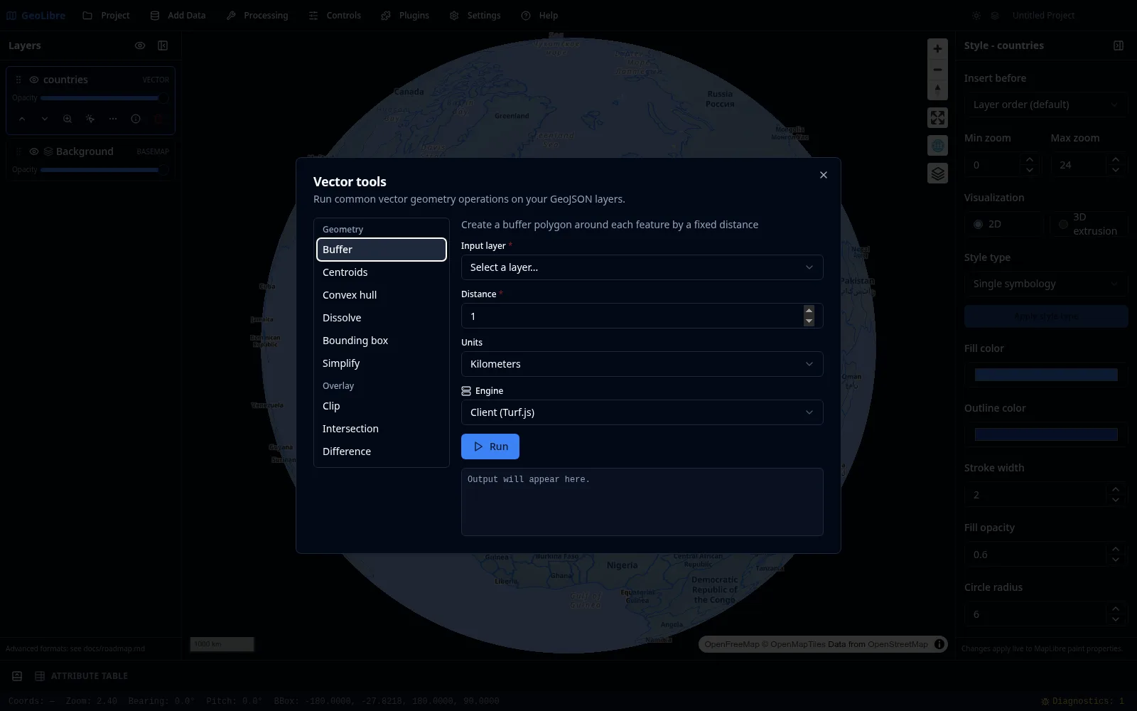
Processing → GeoLibre Toolbox → Vector opens the Vector tools dialog. Pick a tool from the list, choose the input layer and parameters, select an engine, then Run. Output appears as a new layer.
Skipping the dialog
Several of these are also one click away from the Quick analysis submenu. Right-clicking the map runs a buffer or a drive- or walk-time isochrone on the clicked point; the submenu on a layer row runs a buffer, centroids, convex hull, or bounding box over the whole layer. See Right-click quick actions.
Geometry
| Tool | Description |
|---|---|
| Buffer | Create a buffer polygon around each feature by a fixed distance. |
| Centroids | Compute the centroid point of each feature. |
| Convex hull | Compute the convex hull enclosing all features. |
| Dissolve | Merge polygon features into a single geometry, optionally grouped by a field. |
| Bounding box | Compute the rectangular envelope of all features. |
| Simplify | Reduce the number of vertices using Douglas-Peucker. |
| Reproject | Reinterpret a layer's coordinates as a source CRS and transform them to WGS84 so they display in the right place. Needs the Sidecar or Python engine. |
| Explode | Split multipart geometries into single-part features, one per part, keeping the parent's attributes. |
| Aggregate by attribute | Dissolve features sharing an attribute value into one geometry per group, with a summary statistic. |
| Smooth | Round the corners of lines and polygons with Chaikin's algorithm (this adds vertices, unlike Simplify). Z values are preserved. |
| Regular grid | Generate a rectangular grid (fishnet) over the map view, a layer's extent, or a manual bounding box. |
| Voronoi / Delaunay | Build a Voronoi diagram (one polygon per point, clipped to the points' extent) or a Delaunay triangulation from a point layer. |
| Cell-site coverage | Build antenna sector polygons from point sites using azimuth, radius, and beamwidth read from fields or fixed values. |
Overlay
| Tool | Description |
|---|---|
| Clip | Clip the input layer to the area covered by an overlay layer (keeps input attributes). |
| Intersection | Keep only the areas where both polygon layers overlap (merges attributes from both). |
| Difference | Remove the overlay layer's area from the input layer (keeps input attributes). |
| Union | Merge two polygon layers into a single combined geometry (attributes are not preserved on either engine). |
Join
| Tool | Description |
|---|---|
| Spatial join | Attach attributes from a join layer to each input feature based on a spatial relationship (intersects, within, or contains). Choose an inner join to keep only matched features or a left join to keep all input features. Works with any geometry type. |
| Attribute join | Attach attributes from a join layer (a table) onto each input feature where a key field matches — no geometry involved (e.g. join census stats to boundary polygons by FIPS code). One-to-one: the first matching join row wins. Choose which fields to bring over, and an inner join (keep only matched) or left join (keep all input). |
Select
| Tool | Description |
|---|---|
| Select by value | Extract features whose attribute matches a condition into a new layer. Pick a field, an operator (=, ≠, >, ≥, <, ≤, contains, starts with, is empty, is not empty) and a value. Comparisons are numeric when both sides are numbers, otherwise text. |
| Select by location | Extract features by their spatial relationship to a second layer (intersects, within, contains, or disjoint) into a new layer. Works with any geometry type. |
| Random extract | Extract a random subset of features into a new layer, sized by a feature count or a percentage of the input. |
Movement & time
| Tool | Description |
|---|---|
| Trajectory speed | Order points by time per target and connect consecutive fixes into segments carrying distance, duration, and speed. |
| Detect stops | Find where a target dwells: runs of consecutive fixes staying within a distance for at least a minimum duration. One point per stop. |
| Space-time proximity | Find pairs of points close in both space and time (two targets meeting, say). Outputs a line per qualifying pair with the distance and time gap. |
Data quality
| Tool | Description |
|---|---|
| Check validity | Find features with invalid geometry (self-intersecting rings, holes outside shells, …) and mark them on the map. |
| Fix geometries | Repair invalid geometries with ST_MakeValid; valid features pass through untouched. |
| Check topology rules | Validate a layer against topology rules (overlaps, gaps, self-intersections, dangles) and mark each violation. |
| Fix topology | Snap nearly-connected line endpoints, fix dangles, and project points onto lines. Free ends with nothing nearby are left alone. |
Engines
Every vector tool can run on one of three engines, selectable in the dialog:
- Client (Turf.js): runs entirely in the browser. No setup, works offline, and operates on the layer's GeoJSON.
- Sidecar (GeoPandas): runs on the optional Python sidecar for projection-aware results, backed by GeoPandas and Shapely. The dialog falls back to the client engine when the sidecar's optional
vectorextra is not installed. - Python (Pyodide): runs the same GeoPandas/Shapely code as the sidecar, but entirely in your browser via Pyodide — no server, so it works on the web build and the public demo too. The first run downloads the Python runtime once (a few tens of MB, fetched lazily from a CDN, so an internet connection is needed the first time); later runs reuse the warmed-up runtime. Because it shares the sidecar's Python, results match the Sidecar engine. By default the runtime loads from the public jsDelivr CDN, which is a trust assumption: a tampered CDN response would run unverified (Pyodide loads its own
pyodide.asm.js/WASM internally, so a subresource-integrity check on the entry script alone is not sufficient). For production or offline use, self-host the runtime by pointingVITE_PYODIDE_INDEX_URLat a mirrored copy of the Pyodide distribution, which removes the CDN dependency entirely.
See the Vector Analysis tutorial.
Raster
Processing → GeoLibre Toolbox → Raster opens the Raster tools dialog. Most raster tools run on the rasterio Python sidecar: they take a file path in and write a file path out, then add the result to the map. Several also offer a Client (browser) engine that computes on the loaded raster without a sidecar.
Terrain
| Tool | Description |
|---|---|
| Hillshade | Compute a shaded-relief raster from an elevation model. |
| Slope | Compute slope (steepness) from an elevation model. |
| Aspect | Compute aspect (compass direction of the steepest slope) from an elevation model. |
Reproject
| Tool | Description |
|---|---|
| Reproject | Warp a raster to a different coordinate reference system. |
| Resample | Resample a raster to a different pixel size (resolution). |
Clip
| Tool | Description |
|---|---|
| Clip by extent | Crop a raster to a bounding box (in the raster's CRS). |
| Clip by mask layer | Clip a raster to the geometries of a vector mask file. |
Raster to Vector
| Tool | Description |
|---|---|
| Polygonize | Convert a raster band into vector polygons grouped by pixel value. |
| Contour | Generate contour lines from an elevation model. |
Vector to Raster
| Tool | Description |
|---|---|
| Interpolation (IDW / Kriging) | Interpolate a point layer's numeric attribute into a continuous raster surface using inverse distance weighting or ordinary kriging. The output grid spans the points' extent at the chosen pixel size, in the layer's CRS. |
Analysis
| Tool | Description |
|---|---|
| Zonal statistics | Summarize raster values within each polygon of a zone layer. |
| Raster calculator | Evaluate an expression across one or more aligned rasters. |
| Spectral index | Compute NDVI, NDWI, EVI, and other indices from band presets. |
| Reclassify | Map pixel value ranges onto new values. |
| Mosaic / merge | Combine several rasters into one. |
| Focal statistics | Compute a moving-window statistic (mean, min, max, …) over a raster. |
Georeferencing sits at the bottom of the same submenu: it pins a non-georeferenced image to the map with ground control points using a least-squares affine fit, reporting per-GCP and RMS residuals.
See the Terrain Analysis tutorial.
Conversion
Processing → GeoLibre Toolbox → Conversion writes data to cloud-native formats:
| Tool | Description |
|---|---|
| Vector to Vector | Convert between any formats DuckDB's spatial extension supports; input and output formats are detected from the file extensions. The desktop app (sidecar) writes any GDAL format (FlatGeobuf, GeoPackage, Shapefile, KML, GML, SQLite, …); the browser writes GeoJSON, CSV, GeoParquet, GeoPackage, FlatGeobuf, and Shapefile. |
| Vector to GeoParquet | Hilbert-sorted, compressed GeoParquet. |
| Vector to FlatGeobuf | Hilbert-sorted, cloud-optimized, spatially indexed vector. |
| Vector to Shapefile | Hilbert-sorted, zipped ESRI Shapefile (field names truncated to 10 characters). |
| Vector to GeoPackage | Hilbert-sorted GeoPackage for sharing with QGIS/ArcGIS. |
| CSV to GeoParquet | Convert a CSV with coordinates to GeoParquet. |
| Vector to PMTiles | Build a vector tile archive. |
| Raster to PMTiles | Render one raster band through a colormap into a PMTiles archive of Web Mercator PNG tiles. |
| Raster to COG | Write a Cloud-Optimized GeoTIFF. |
Every one of these has a client-side engine, so all of them work in the browser and on the Mac App Store build. On desktop they run on the Python sidecar instead, which reads and writes native file paths and, for Vector to Vector, can write any format GDAL supports rather than the browser's shorter list. Raster to PMTiles is the exception: it has no sidecar endpoint at all and always runs in WebAssembly. The dialog names the engine it is about to use in its status line.
The sidecar can also confine conversion inputs and outputs to an allowlist of directories, set through GEOLIBRE_CONVERSION_ROOTS. It is unset on the desktop app, where the paths are your own filesystem and there is nothing to confine. The Docker image sets it, because there the sidecar is reachable same-origin through the nginx proxy and must not be able to read or overwrite arbitrary container paths. See Self-Hosting.
Not the same as Processing → Conversion
The bare Conversion submenu higher up the menu is the Whitebox toolbox's conversion category (format and raster/vector conversion tools from the WASM catalog). The dialogs in this table live under GeoLibre Toolbox → Conversion. See Two toolboxes in one menu.
Network
Processing → GeoLibre Toolbox → Network runs routing analysis against a Valhalla server (the public FOSSGIS instance by default, so the coordinates you submit leave your device; self-hosted deployments can point at their own, see Self-Hosting).
| Tool | Description |
|---|---|
| Isochrone / service area | Polygons reachable within given travel times from one or more origins. |
| OD cost matrix | Travel time and distance for every origin-destination pair between two point layers. |
| Sequential route (directions) | Route through a set of stops in order, with turn-by-turn directions. |
Spatial Statistics
Processing → GeoLibre Toolbox → Spatial Statistics runs pattern analysis on a point or polygon layer and adds the result to the map.
| Tool | Description |
|---|---|
| Global Moran's I | A single measure of whether a numeric attribute is clustered, dispersed, or random across the layer. |
| Local Moran's I (LISA) | Per-feature clustering: high-high, low-low, and spatial outliers. |
| Getis-Ord Gi* hotspots | Per-feature hot and cold spots with significance levels. |
| Average nearest neighbor | Whether a point pattern is more clustered or dispersed than random. |
| Kernel density (heatmap) | A continuous density surface from a point layer. |
| Emerging Hot Spot | Hot-spot trends over time from a space-time cube. |
DGGS
Processing → GeoLibre Toolbox → DGGS works with discrete global grid systems (H3, S2, A5, DGGRID, DGGAL).
| Tool | Description |
|---|---|
| DGGS Generator | Fill an area with DGGS cells, from a layer's geometry or extent, the map view, or a manual bounding box. |
| DGGS Binning | Aggregate a point layer into DGGS cells (count, or sum/mean/min/max of a numeric field). |
| DGGS Compact | Compact DGGS polygon cells, or expand them to a uniform resolution. |
Geocode Addresses, Batch & Models
Two more entries sit below the separator in the GeoLibre Toolbox submenu:
- Geocode Addresses turns a table of addresses into a point layer.
- Batch & Models runs one tool across many input layers (Batch), or chains tools so each step's output feeds the next and saves the chain with the project (Models). Both modes draw on the Vector tools above and run on the client engine.
AI Segmentation, Object Detection, Segment Everything
- AI Segmentation turns imagery into vector features with segment-geospatial (SamGeo) and Meta's SAM 3 model: choose a GeoTIFF, type a text prompt ("trees", "buildings") or run automatic segmentation, and the resulting polygons are added as a new layer. It runs the model in a separate
samgeo-apiserver (a GPU is recommended) that the sidecar proxies. See the dedicated AI Segmentation page for setup and usage. - Object Detection and Segment Everything run client-side in the browser on
onnxruntime-web, so they need no sidecar and stay available on the web build and on mobile.
Whitebox Toolbox
Processing → Whitebox Toolbox opens the geoprocessing toolbox: 1,000+ tools covering vector, raster, remote sensing, hydrology, terrain, LiDAR, conversion, network, and projection analysis.
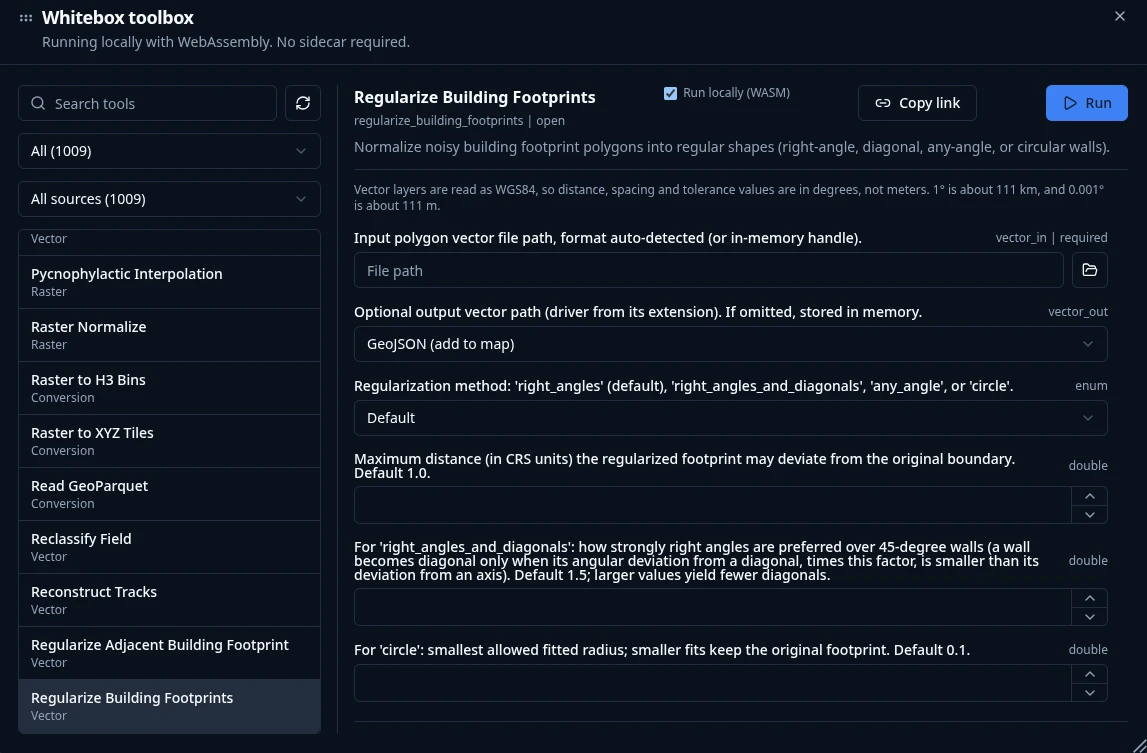
The tools come from the Whitebox Next Gen suite together with GeoLibre's own WASM tools from geolibre-rust, which the dialog mixes into the same catalog (use the source dropdown to filter to one or the other). The category and subcategory names, and the tool names themselves, come straight from the tool manifests and are generated automatically, so they follow upstream naming rather than GeoLibre's.
Where the tools run
They run in the browser, through a WebAssembly runtime with raster and vector I/O — no Python sidecar, no server, and no data leaving your machine. That means the full toolbox is available on GeoLibre Web and on Android and iOS, not just the desktop app.
The Run locally (WASM) checkbox controls the engine:
- Checked runs the tool in WebAssembly on the layer or file you pick. This is the default in the browser build, where no sidecar can be started. The Mac App Store build has no sidecar to switch to at all, so the checkbox does not appear there — WebAssembly is the only runtime.
- Unchecked sends the job to the Python sidecar instead. This is the default on desktop, where the sidecar is available. The sidecar can read native file paths that the in-browser runner cannot fetch, and is the better choice for batch runs across a directory of files on disk.
Either way the tool list is the same; only the executing engine changes.
Finding and running a tool
- Search by name at the top of the tool list, or narrow with the category and source dropdowns.
- Browse by category without opening the dialog at all: the Processing menu has a submenu per category (Conversion, Hydrology, LiDAR, Network, Projection, Raster, Remote Sensing, Terrain, Vector) with nested subcategory submenus, including the
GeoLibre (WASM)subheading for GeoLibre's own tools. Picking a tool opens the dialog with it preselected. The catalog is bundled offline, so the menu works with no network. - Fill in the form — the dialog builds it from the tool's own parameter manifest, with a file picker for path inputs and an output-format dropdown for vector outputs. Parameters that are ground distances get a metric unit picker.
- Run, and the output is added to the map. Raster outputs are Cloud Optimized GeoTIFFs.
Share a link to a tool
Copy link builds a URL with a ?tool= parameter that reopens the app with that tool preselected and its form pre-filled — handy for documentation, teaching, and bug reports.
Every run is recorded in Processing → History, which re-runs any entry with one click and copies the equivalent Python code. Both toolboxes write to the same history.
Planetary Computer and Earth Engine
The Processing menu also opens the Planetary Computer and Earth Engine panels for browsing and loading cloud datasets. See Data Integrations.
The Python sidecar
The raster tools, the sidecar conversion tools, and the optional GeoPandas vector engine use a local FastAPI sidecar that the desktop app starts on demand. The Whitebox Toolbox can optionally use it too, but does not need it — it runs in WebAssembly by default. The vector tools' client engine and the browser-based conversions need no sidecar either. See Getting Started for setup and Reference → Architecture for how it works.
Browser vs desktop
The Whitebox Toolbox, the client-side vector tools, and every Conversion tool run in the browser. Vector to Vector's full any-format output and the full raster tool set require the desktop app and the Python sidecar.